Studies in Composing Hydrogen Atom Wavefunctions
Lance J. Putnam,1, JoAnn Kuchera-Morin2, Luca Peliti3, 4
1(Academic, composer), Department of Architecture, Design and Media Technology, Aalborg University, Sofiendalsvej 11, DK-9200 Aalborg (Denmark). E − mail:
lp@create.aau.dk
2(Academic, composer), Media Arts and Technology, University of California, Santa Barbara, Santa Barbara, CA, 93106-6065 (USA). E − mail:
jkm@create.ucsb.edu
3(Academic), Dipartimento di Fisica, Università “Federico II”, Complesso Monte S. Angelo, 80126 Napoli (Italy). E − mail:
peliti@na.infn.it
4INFN, Sezione di Napoli, Complesso Monte S. Angelo, 80126 Napoli (Italy)
We present our studies in composing elementary wavefunctions of a hydrogen-like atom and identify several relationships between physical phenomena and musical composition that helped guide the process. The hydrogen-like atom accurately describes some of the fundamental quantum mechanical phenomena of nature and supplies the composer with a set of well-defined mathematical constraints that can create a wide variety of complex spatiotemporal patterns. We explore the visual appearance of time-dependent combinations of two and three eigenfunctions of an electron with spin in a hydrogen-like atom, highlighting the resulting symmetries and symmetry changes.
1 Introduction
We attempt to represent the state of a quantum system and its evolution in an immersive integrated environment, as a way to obtain, for the scientist, a better intuitive understanding of quantum reality and to produce, for the composer, a powerful medium for aesthetic investigations and creative expression. Specifically, the hydrogen-like atom is important for scientists as it accurately describes some of the fundamental quantum mechanical phenomena of nature. For the composer, it supplies a set of well-defined mathematical constraints that can be adjusted to create a wide variety of spatiotemporal structures.
Making such a quantum system perceptible is of utility to both the scientist and artist. First of all, doing so renders the abstract mathematical system into a format that can be experienced in a way that is more intuitive and visceral. Such a representation will not necessarily contribute to our understanding of the Hilbert space in which the atom lives, but can give a feeling of this abstract space in the more familiar space we all live. Second, perceptualizing the atom can assist in understanding emergent patterns, flows, symmetries and dynamics when multiple hydrogen-like wavefunctions are mixed in superposition. It can be difficult to represent these complex phenomena in one’s head from the mathematical equations alone.
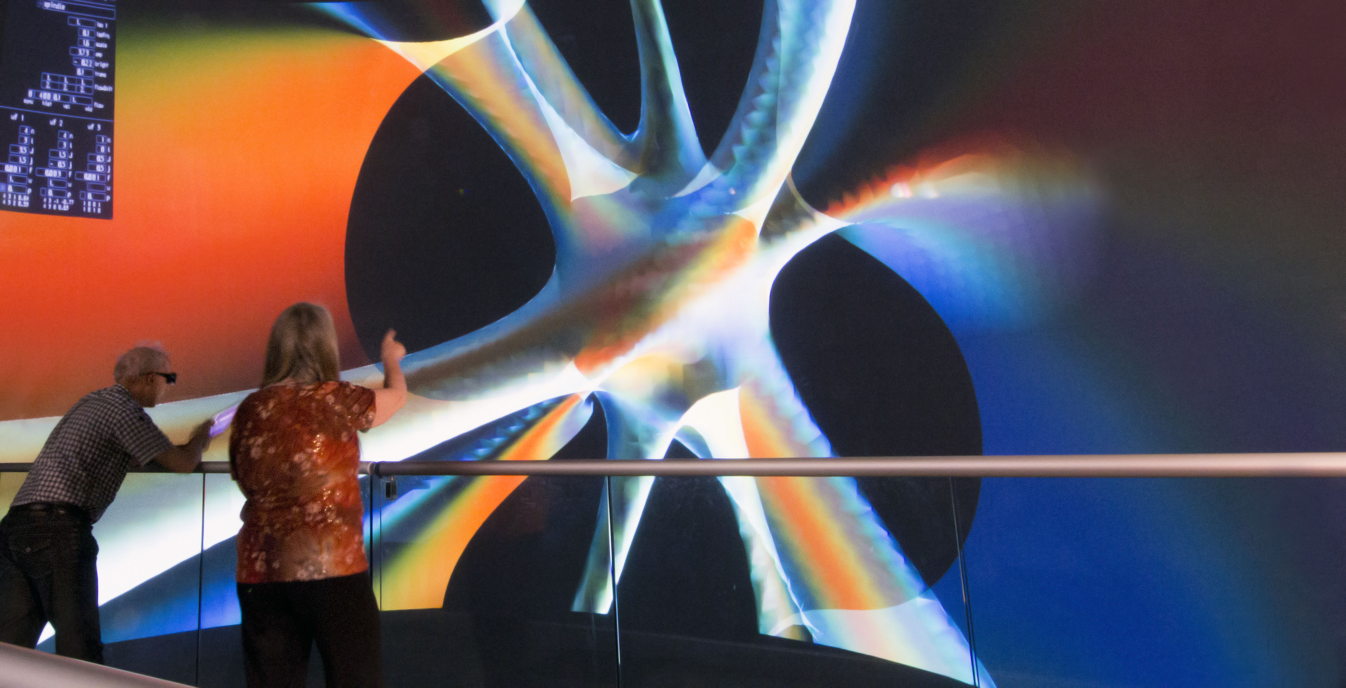
In order to represent the wavefunctions, we use the AlloSystem software framework
[1] to facilitate the interactive visualization of this information and the AlloSphere
[2], a three-story, spherically-shaped virtual reality environment, to allow full immersion in the data. The AlloSphere not only can provide an intuitive understanding of the hydrogen-like atom through perception
[14], but also permits observation of multiple levels of structure in a way that is more natural than a flat display (wall) (Figure
1↓). The hydrogen-like atom is a test bed for the AlloSystem software and AlloSphere instrument and a necessary prerequisite towards representing more complex and nuanced quantum systems. We decided, as a first step, to represent the wavefunctions visually as this appears to be more easily understood than, for instance, translating them into sound.
2 Related Work
Over the past century, many approaches have been taken to visualizing atomic orbitals, mostly for didactical purposes. The first visualizations of hydrogen atom orbitals were made in 1931 using time exposure photography of the motions of a modified mechanical lathe
[7]. Berndt Thaller has done extensive work on the visualization of quantum mechanical states, in particular in three-dimensional systems
[4, 3] and hydrogen-like atoms, by means of several visualization techniques. However, the stress laid on the temporal evolution of the wavefunctions is comparatively limited.
Several interactive tools have been made that visualize dynamic mixtures of hydrogen-like atom wavefunctions in real-time. Falstad’s
Hydrogen Atom Applet [17] displays a volume rendering of mixtures of any number of orbitals, but only with low energy levels. Dauger’s
Atom in a Box [6] also employs volume rendering and allows mixing of up to eight wavefunctions with relatively high energy levels. These tools, however, do not represent wavefunctions with spin.
The time evolution of an arbitrary initial wavefunction is visualized by a software package developed by Belloni and Christian
[16, 15]. The method applies to one-dimensional system with a purely discrete spectrum. The wavefunctions are projected on the eigenfunctions of the system and the subsequent evolution is obtained by evolving the coefficients of the decomposition. While the subtleties of quantum-mechanical evolutions are well captured by this software, its application to higher-dimensional systems would be quite difficult.
Artistically, we identify our work closely with John Whitney’s concept of digital harmony
[11] in applying harmonics and other musical notions, such as scales and transitions of curves, to visual composition. Julian Voss-Andreae’s quantum sculptures
[12] are also relevant being visual interpretations of quantum mechanics, however, are more conceptual in nature and do not give a picture of the complex dynamics of quantum systems.
3 Conceptual Framework
Our conceptual framework is based on a particular process of musical composition, namely, the organization of frequencies and pitches, transposed from the sound domain to the visual domain. More specifically, we propose working with wavefunctions in a similar way to how a composer works with musical tones in creating a larger work.
Quantum mechanics dictates that the evolution of a quantum state is realized by a process that closely resembles additive synthesis in music. A general time-dependent quantum state is obtained by the superposition of a number of wavefunctions representing stationary states, the eigenfunctions, multiplied by periodically varying coefficients. The eigenfunctions correspond to the simple sounds that add together to form the complete synthesized sound. Their superposition produces the complex spatiotemporal pattern described by the time-dependent wavefunction.
In the following, we present several concepts in musical composition and physics that support our analogy between wavefunctions and musical tones.
3.1 Compositional Process
Music carries meaning on several time-scales, from individual timbres and pitches (foreground) to short melodies and rhythms (middle-ground) all the way up to large-scale form and structure of a work (background), each engaging distinct perceptual and cognitive processes. Typically, when composers start to realize a piece of music they either have a big idea at the macro-level (a large structure that they want to unfold), or they start with something at the micro-level such as a small group of notes. One strategy composers use to master their data in unfolding a piece is to work at a middle-ground level, that is, controlling the larger structure at the background while unfolding the microstructure at the foreground
[8]. Also, in predicting local motion in self-generative music from the microstructure, a middle-ground-to-foreground approach may aid in local directional choices. In Xenakis’ compositional approach, local events are decided randomly, however these events are constrained by clearly articulated probability distributions
[10]. This approach is similar to the relationship between the deterministic Schrödinger evolution and probabilistic measurement process in quantum mechanics.
Sketching is a technique used in composition where a composer will try out various scenarios of harmonic structures in creating a work. Typically a composer will write a series of studies called études, that are part of the sketching process. The sketching process is hierarchical in that a rough draft of the structure is sketched, and then various parts are filled in at the micro-level, which will cause adjustments at the macro-level. This is the middle-ground area that functions as the pendulum between the micro and macro layers. Since this process is hierarchical, it can be applied at the level of adding frequencies together to build larger structures.
Our initial approach in composing with the hydrogen-like atom is to start with a middle-ground which we identify as interference patterns. Thus, we can experiment with various combinations of multiple wavefunctions that are scientifically correct and we find aesthetically pleasing. We begin the process with sketching---a series of studies mixing multiple eigenfunctions together. The studies range from the physically-motivated to the open-ended, exploring beating and complex interference patterns such as fine-splitting. Thus, we are creating the basic musical alphabet by mixing the multiple eigenfunctions together with certain chosen characteristic frequencies.
3.2 Eigenfunctions
We employ eigenfunctions as our basic units of composition. Eigenfunctions are identified by a set of quantum numbers that determine the particular shape of the eigenfunction in space (Section
3.5↓) as well as its frequency of evolution through time. Controlling the effect of the quantum numbers on the visual pattern that is produced is the basic step in the creation of a satisfactory composition.
A quantum state represented by a single eigenfunction evolves through a space-independent phase factor that changes periodically in time with its characteristic frequency. Thus, the spatial distribution of an eigenfunction’s magnitude does not change with time. Additionally, two different eigenfunctions can share the same characteristic frequency. An eigenfunction is analogous to a normal mode in a pipe while a characteristic frequency is analogous to a pure tone.
Eigenfunctions can be placed in superposition to create a wavefunction (see Appendix). Such wavefunctions generally have more complex properties than their constituent eigenfunctions. This is analogous to how more complex tones can be built from simple tones, as done with an organ, or from musical voicing and chorusing. These emergent complexities can often be identified with interference patterns.
3.3 Interference Patterns
From an artistic standpoint, the phenomenon of interference is interesting as it allows complex emergent patterns to be constructed from an “alphabet” of simple parts. Strong interference patterns occur when two or more waveforms with similar frequencies are superposed.
An elementary form of interference, beating, occurs when two sinusoids with similar frequencies are summed together.Musically speaking, beating effects can enrich static tones by imposing an evolution of timbre relative to pitch that is an order of magnitude slower. To obtain a complex beating pattern, one can mix two waveforms with the same timbre, but slightly different pitch. This technique called celeste was devised by early organ builders to enrich the sound of individual notes. Similarly, mixing two eigenfunctions produces a spatial pattern that evolves periodically in time, with a frequency equal to the difference between the characteristic frequencies of the eigenfunctions.
While celeste produces a more complex time evolution of a waveform, the effect is strictly periodic in both the time and frequency domains. To alleviate these periodicities, one must mix three or more waveforms together. A wavefunction obtained by superposing three or more eigenfunctions produces a pattern that in general never repeats itself. Interestingly, fine-splitting in an atom can be represented with a mixture of three eigenfunctions.
3.4 Hydrogen-like Atom
A hydrogen-like atom consists of a single particle of mass
m subject to a central force whose potential is inversely proportional to the distance from the nucleus. The characteristic frequencies given by this spectrum rapidly become smaller, leading to slower evolution, as the principal quantum number
n increases. They depend only on
n and
J, and the
J dependence (a spin-orbit coupling effect) is very weak. The
J dependence produces the fine-splitting of spectral lines, discussed in section
4.3↓.
The hydrogen eigenfunctions provide sufficient complexity to be used as building blocks for our composition. Using hydrogen rather than, say, the harmonic oscillator eigenfunctions is analogous to using an organ to create music rather than individual sine waves. This lends sufficient interest in using the compositional process of mixing waveforms to build chords that act as building blocks for visualization. However, the fact that a great number of eigenfunctions exhibit the same characteristic frequency strongly reduces the possibilities to obtain beating patterns. We took therefore the liberty to assign frequencies to the eigenfunctions in an arbitrary way.
3.5 Geometric Properties of the Eigenfunctions
To assist in composition, it is useful to understand the geometrical properties of the eigenfunctions. It is convenient to start from the eigenfunctions of the spinless electron identified by the quantum numbers
(n, ℓ, m). They are characterized by a number of windings, shells and stacks, i.e., elementary patterns relative to a sphere with a north and south pole on the
z-axis (Table
1↓). Windings are the cycles made by the phase of the eigenfunction in making one loop around the
z-axis, stacks are the parallel slices running perpendicular to the
z-axis, and shells are the concentric regions separated by spherical surfaces where the eigenfunction vanishes.
|
Parameter
|
|
|
Range
|
|
Winding number
|
nw
|
: = m
|
…, − 2, − 1, 0, 1, 2, …
|
|
Number of stacks
|
ns
|
: = ℓ − |m| + 1
|
1, 2, …
|
|
Number of shells
|
nr
|
: = n − ℓ
|
1, 2, …
|
Table 1 Geometric properties of spinless eigenfunctions in terms of quantum numbers.
The eigenfunctions of the electron with spin are obtained by superimposing two spinless eigenfunctions with the same values of n and ℓ, but values of m differing by 1. Thus, one eigenfunction has one more winding and one less stack than the other. As the spin eigenfunction is identified by a four-dimensional spinor at each point in space, rather than a complex number as in the spinless version, it cannot be simply described in terms of windings and stacks. However, in general, higher quantum numbers correspond to more spatially extended and varying eigenfunctions.
4 Studies
Our studies aimed to explore the emergent structures and dynamics resulting from mixing together multiple eigenfunctions. Due to the vast number of possible eigenfunction combinations, we decided to limit our scope, for now, to mixtures of only two or three eigenfunctions.
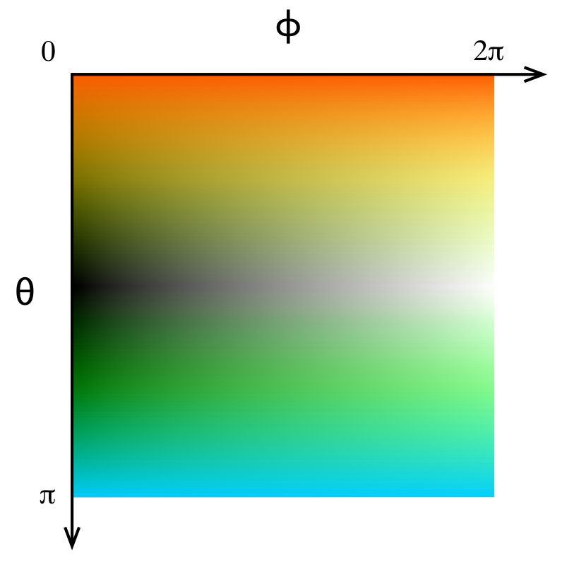
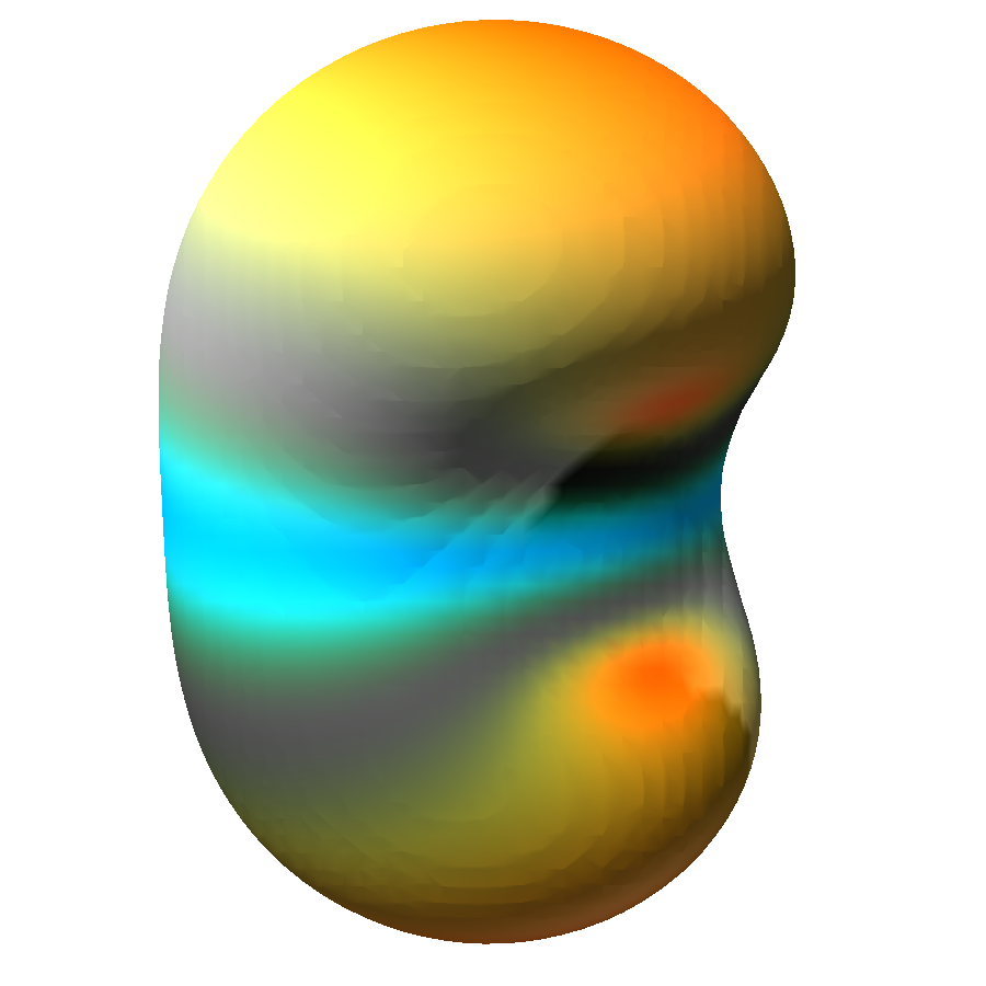
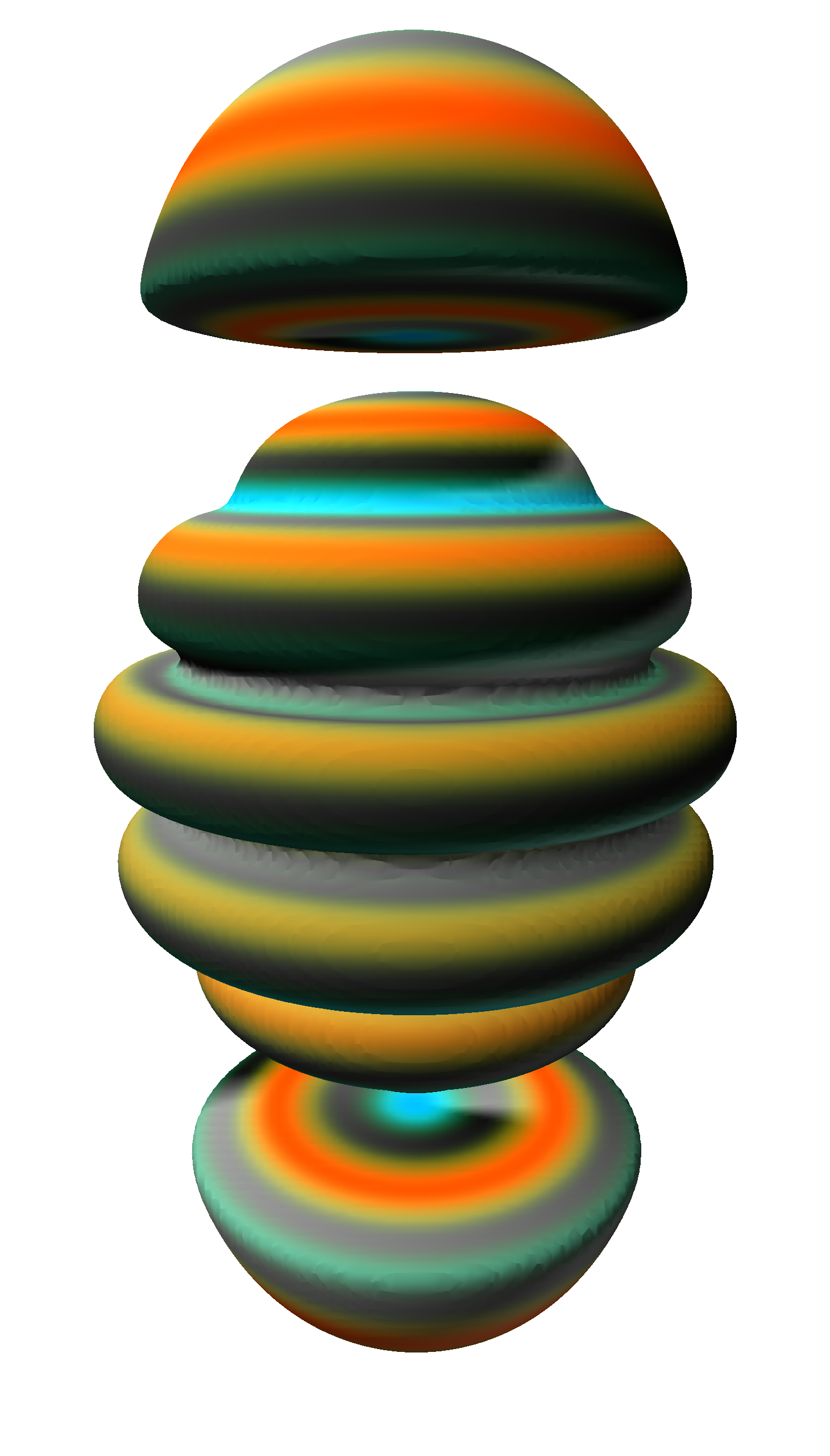
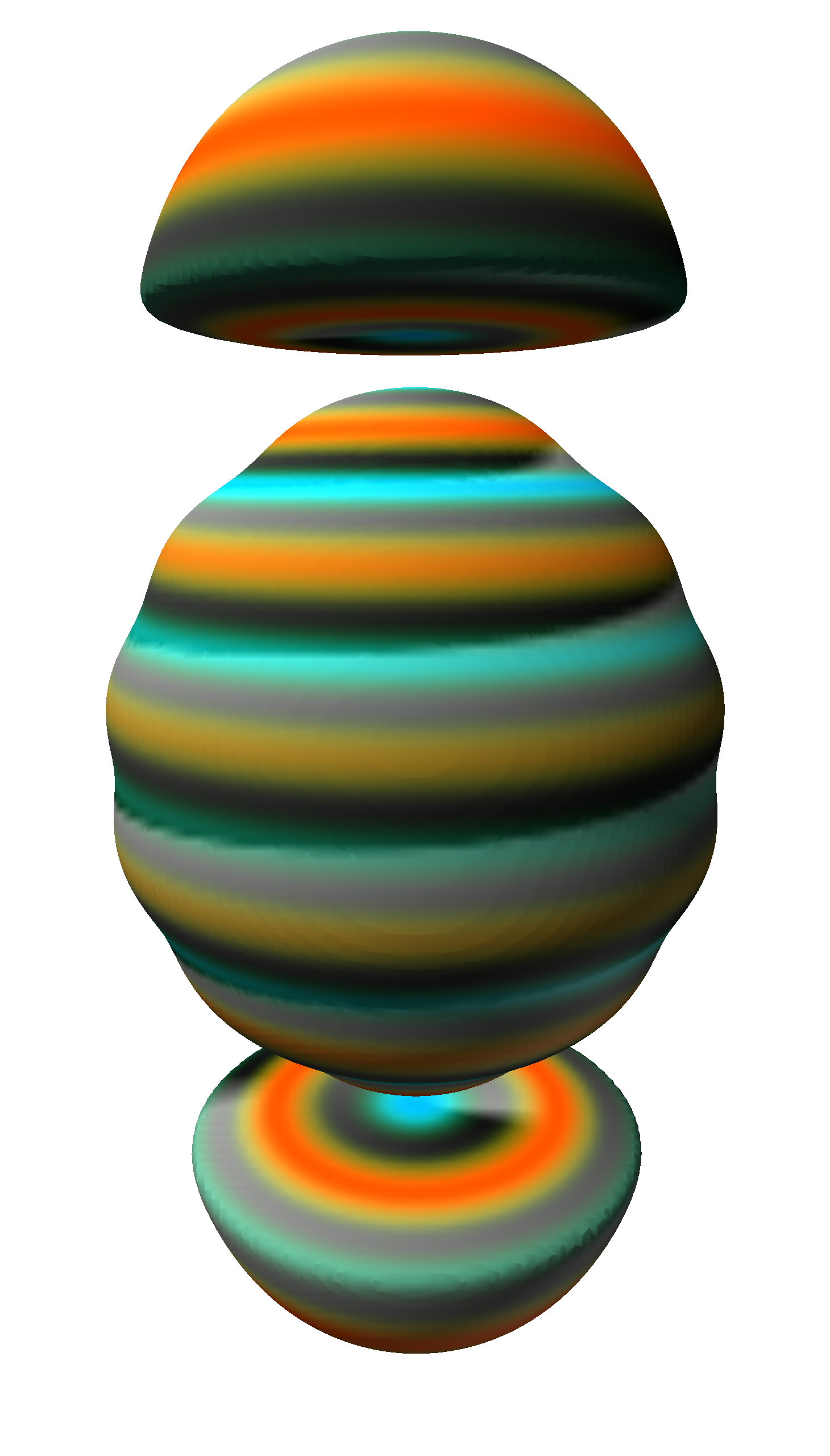
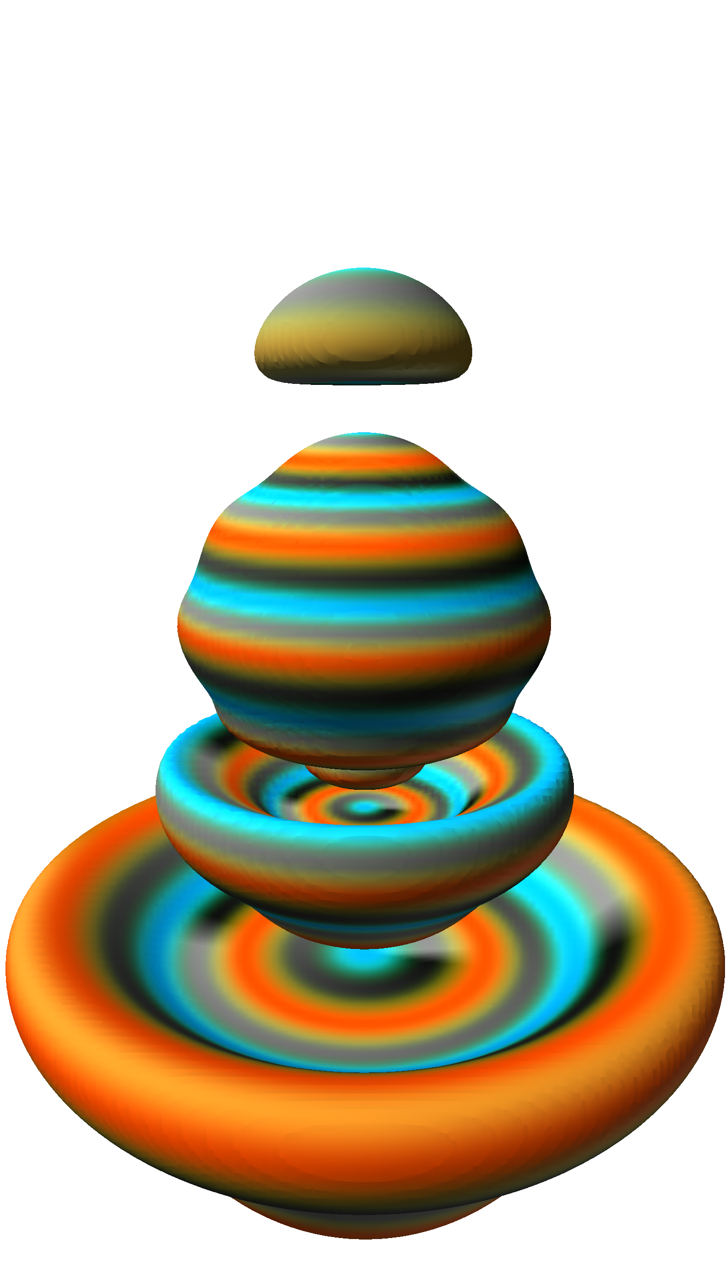
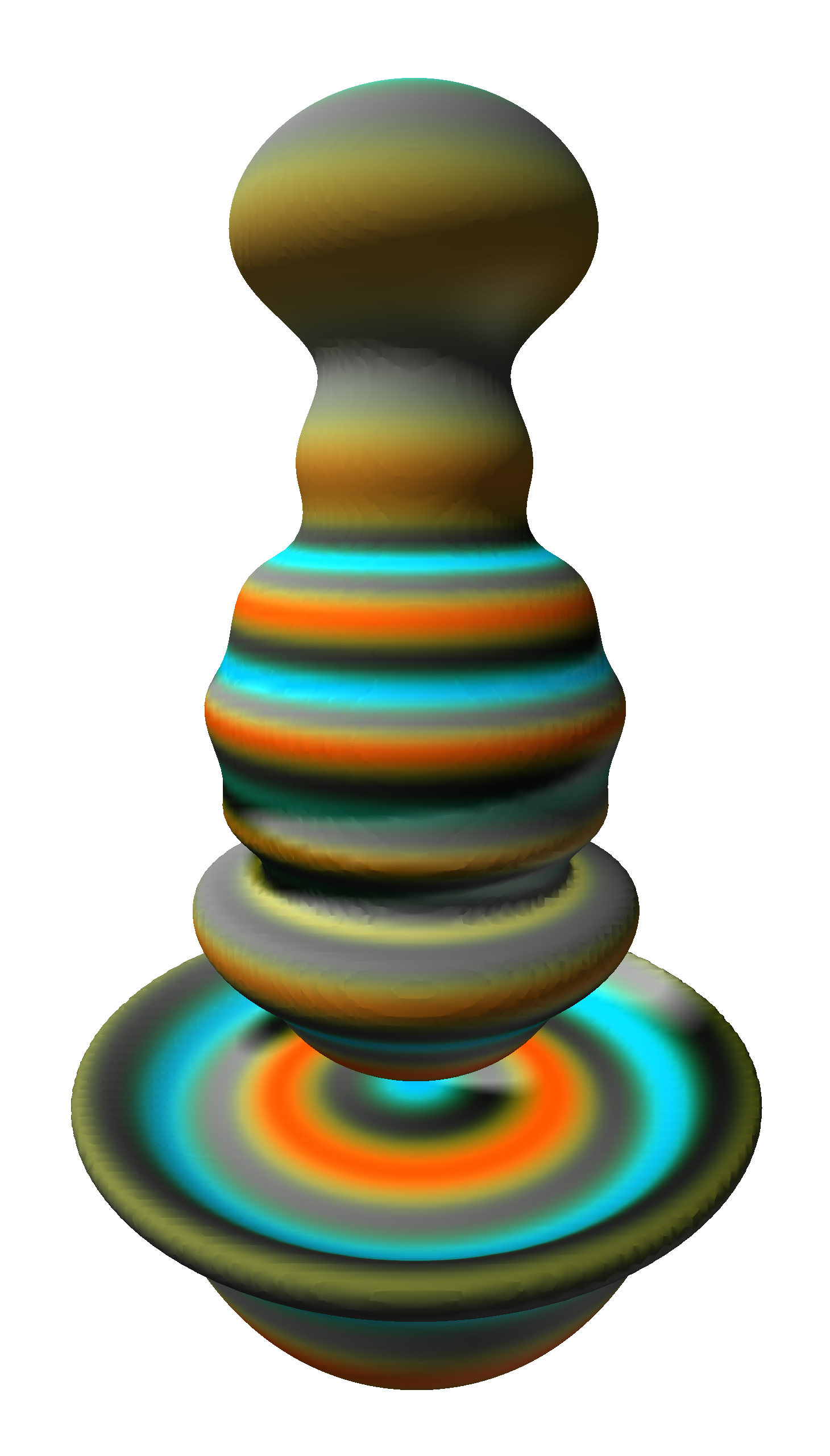
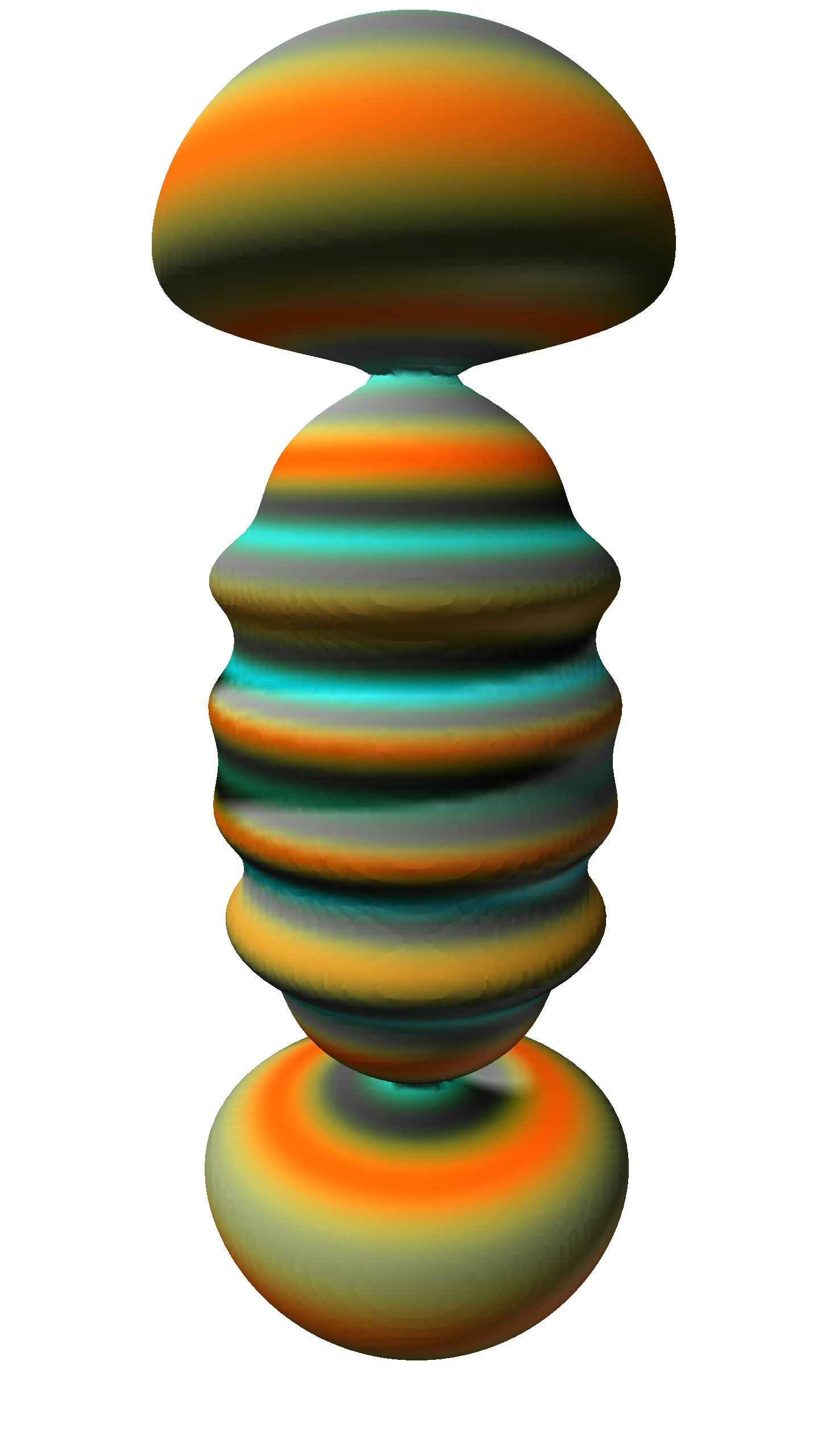
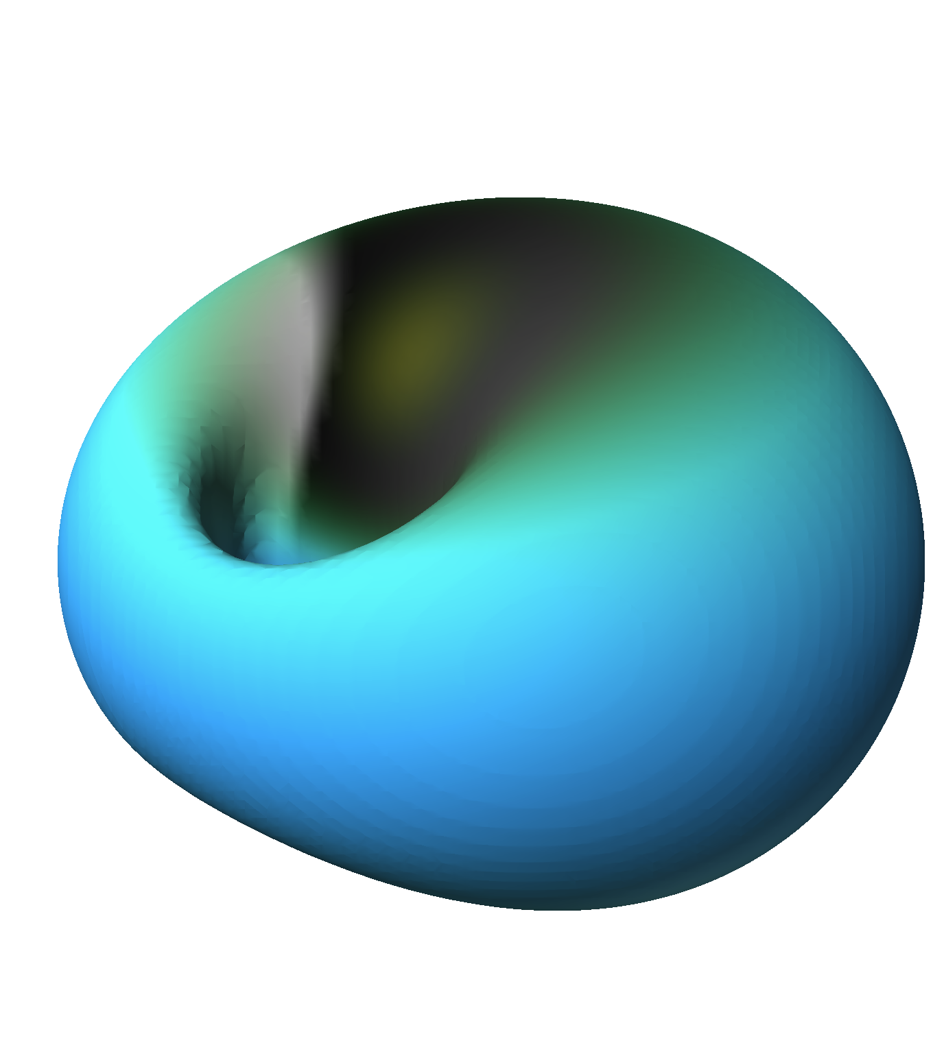
To visualize a wavefunction with spin, we use a color-mapped isosurface as we find it gives a clear picture of the wavefunction’s overall magnitude and phases. The surface is drawn at a particular value of the wavefunction magnitude
|Ψ|. The surface is colored according to the spin vector phases
θ (spin-up/-down state) and
φ (relative phase). We map
θ to hues going between orange (spin up) and cyan (spin down) and
φ to a grayscale gradient. The grayscale gradient is discontinuous revealing an abrupt cut where the phase completes the cycle
[9]. The cuts are more indicative than a smooth mapping and helpful in distinguishing between the two different phases. The hues and grays are interpolated between according to the proximity of the spin vector to the equator; more hue near the poles and more gray near the equator (Figure
2↓).
4.1 One Eigenfunction
There are already a number of programs allowing for the visualization of single eigenfunctions of the hydrogen-like atom
[18][5]. Since the time dependence of a single eigenfunction only appears in an overall phase factor, it leads to a completely time-independent image in our representation, where the overall phase factor is neglected. Thus the representation of single eigenfunctions lies outside the scope of the compositional process, and we did not investigate it systematically. Indeed, a number of software projects have already tackled the problem of visualizing the eigenfunction of the hydrogen-like atom, both in its spinless version and in the one with spin
[4, 3]. We are more interested in the time-dependent patterns one obtains by mixing two or more eigenfunctions.
4.2 Two Eigenfunctions
4.2.1 General Patterns
When mixing two eigenfunctions, we already observe a wide variety of patterns. The patterns evolve periodically either by changing shape or by rotating, with a frequency proportional to the energy difference of the eigenstates. In order to make this evolution visible, we arbitrarily lower this frequency. Fortunately, these patterns can be classified into a handful of general categories of shapes and dynamics that can be related to the quantum numbers.
We observed the following mutually exclusive types of dynamics with respect to the wavefunction magnitude and spin:
-
No change over time.
-
Rotation around the z-axis (with possible exception of relative phase).
-
Beating of magnitude
-
isotropically,
-
radially, and
-
along the z-axis.
Type 1 dynamics involve no change in the wavefunction magnitude and spin vector. This occurs whenever the characteristic frequencies
ϵν are equal. Type 2 dynamics display a periodic rotation of the wavefunction around the
z-axis. There is also a periodic change in the relative phase of the spin at the same rate. One can interpret this rotation as an angular traveling wave. Type 3 dynamics are the most interesting and consist of beating effects that may involve a change in the shape of the wavefunction magnitude. The primary constraint on type 3 dynamics is that the
js are equal. Beating patterns are rotationally invariant around the
z-axis. For type 2 and 3 dynamics, the rate of change of the wavefunction magnitude is equal to the difference between the two characteristic frequencies. The exact constraints on the eigenfunction parameters are given in Table
2↓.
|
Case
|
n
|
ℓ
|
J
|
j
|
ϵν
|
Comments
|
|
1
|
|
|
|
|
=
|
|
|
2
|
|
|
|
≠
|
≠
|
|
|
3(a)
|
=
|
=
|
=
|
=
|
≠
|
|
|
3(b)
|
≠
|
=
|
=
|
=
|
≠
|
|
|
3(c)
|
|
ℓ1 + ℓ2 odd
|
|
=
|
≠
|
Asymmetric w.r.t xy-plane
|
|
3(c)
|
|
ℓ1 + ℓ2 even
|
≠
|
=
|
≠
|
Symmetric w.r.t xy-plane
|
Table 2 Parameter constraints for two-eigenfunction dynamic types. Empty cells indicate no dependence on the parameter.
The shape of the wavefunction magnitude is limited to a few particular types of point group symmetries. The difference between the js is the order of dihedral symmetry around the z-axis, i.e., the number of planes of reflection passing through the z-axis. When the js are equal, there are an infinite number of reflection planes and thus the shape is rotationally invariant around the z-axis. For non-beating wavefunctions, the shape exhibits either reflection or rotation-reflection symmetry with respect to the xy-plane. The rules are
ℓ1 + ℓ2 + j1 + j2 → ⎧⎨⎩
even
rotation-reflection
odd
reflection
Changing
J does not effect symmetry type since it only changes the eigenfunction weights. Complex wavefunctions displaying the two types of symmetry are shown in Figure
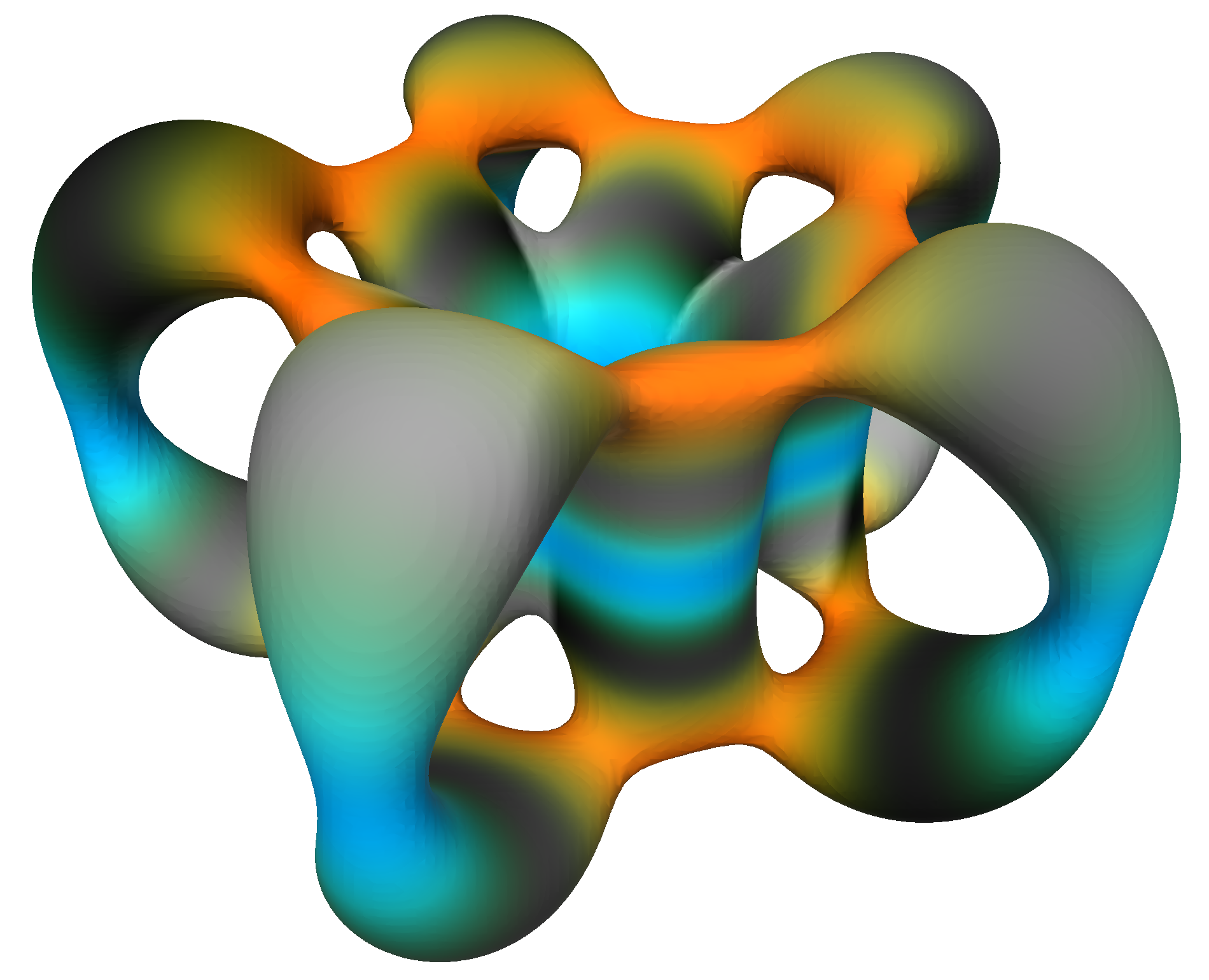
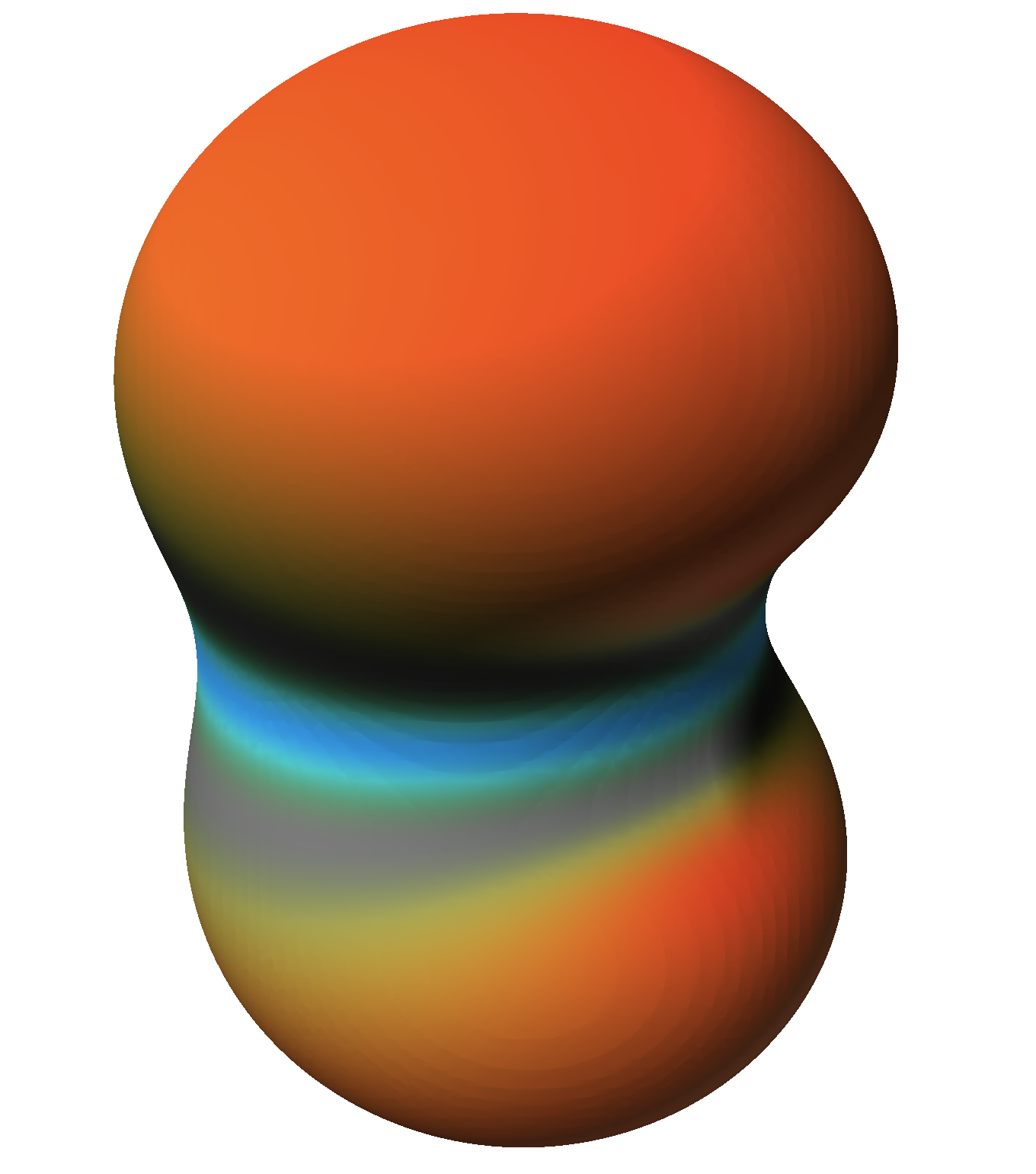
3↓.
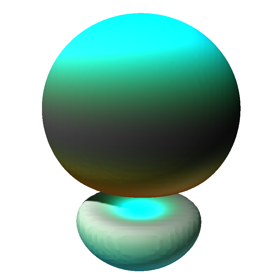
4.2.2 Light-emitting Combinations
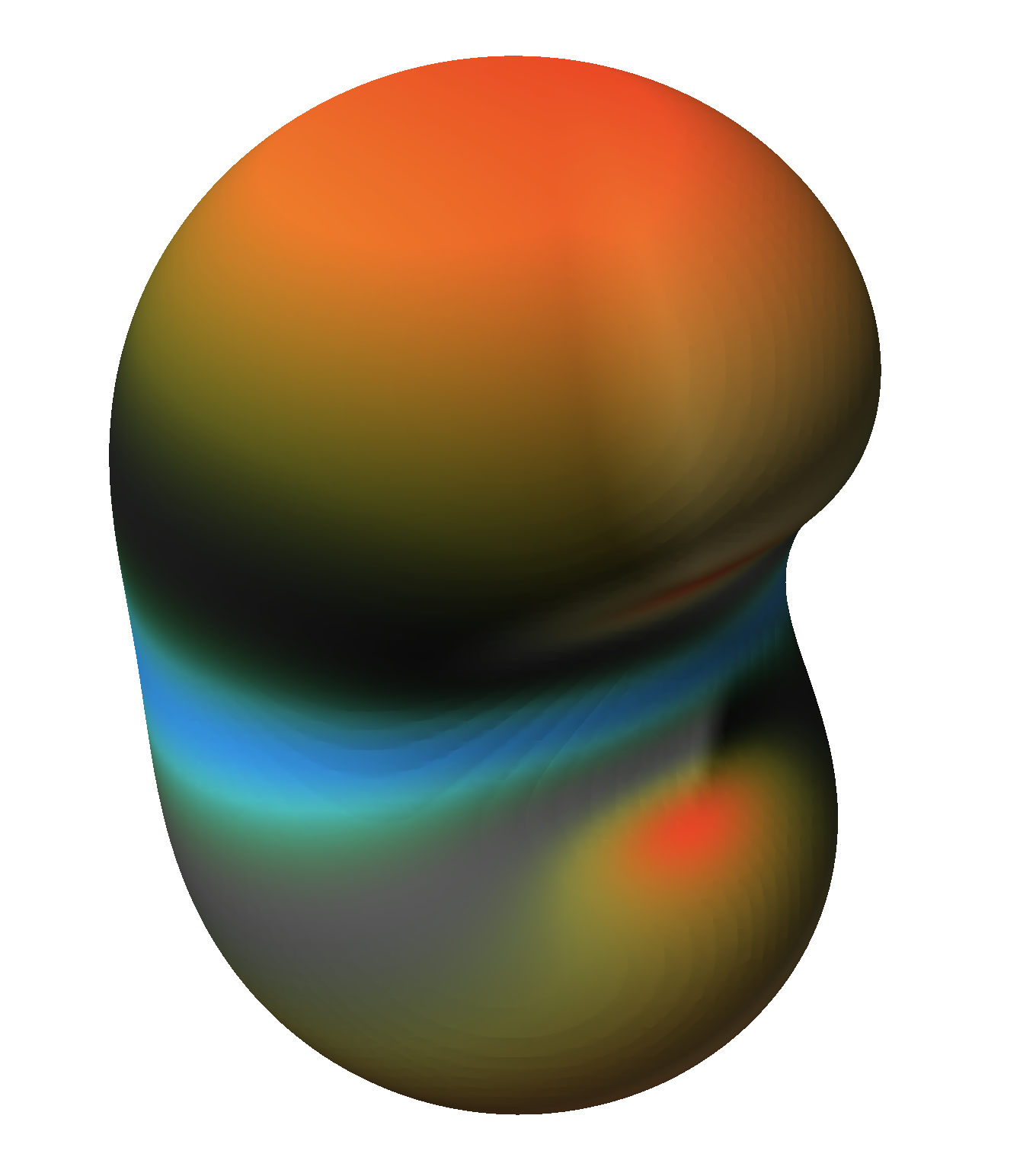
Although we cannot represent the process of light emission in our system, we can illustrate it through a superposition of eigenfunctions which satisfy the selection rules (see Appendix). This leads to a number of interesting wavefunctions which periodically change at a rate equal to the frequency of the emitted photon. Figure
4↓ shows all such superpositions which can be built out of the lowest values of
n. Interestingly, they include all the non-trivial types of dynamics and three distinct types of spin distributions.
When the
n values are very different, one sees a relatively smaller radial interference. Indeed, most of the interference takes place in the region occupied by the eigenfunction with the smaller
n value. More complex patterns can be found when the
n values are close and larger (Figure
5↓).
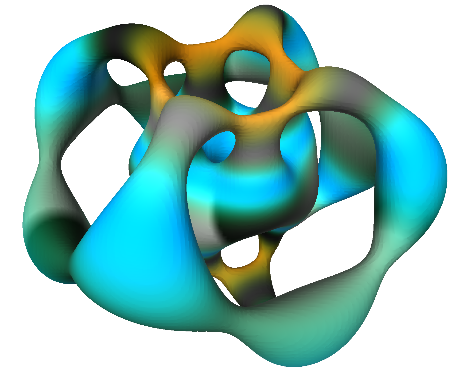
It appears that the only shapes for light emission superpositions are rotationally invariant around z or have reflective symmetry with respect to the xy plane. None exhibit rotation-reflection symmetry.
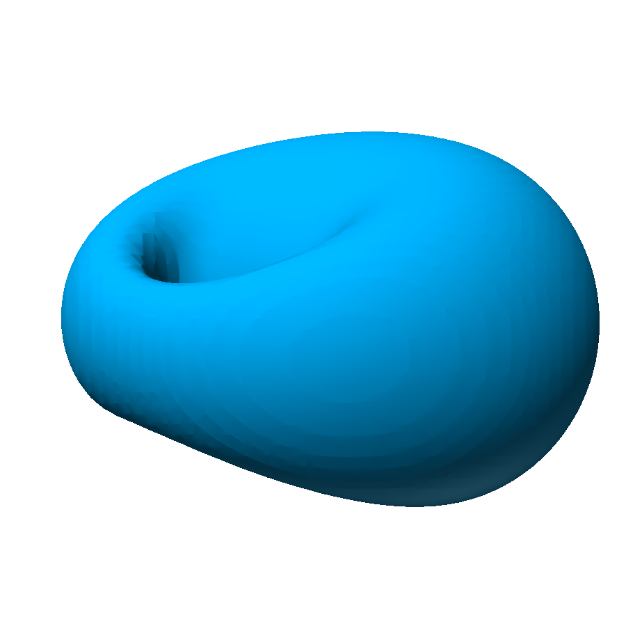
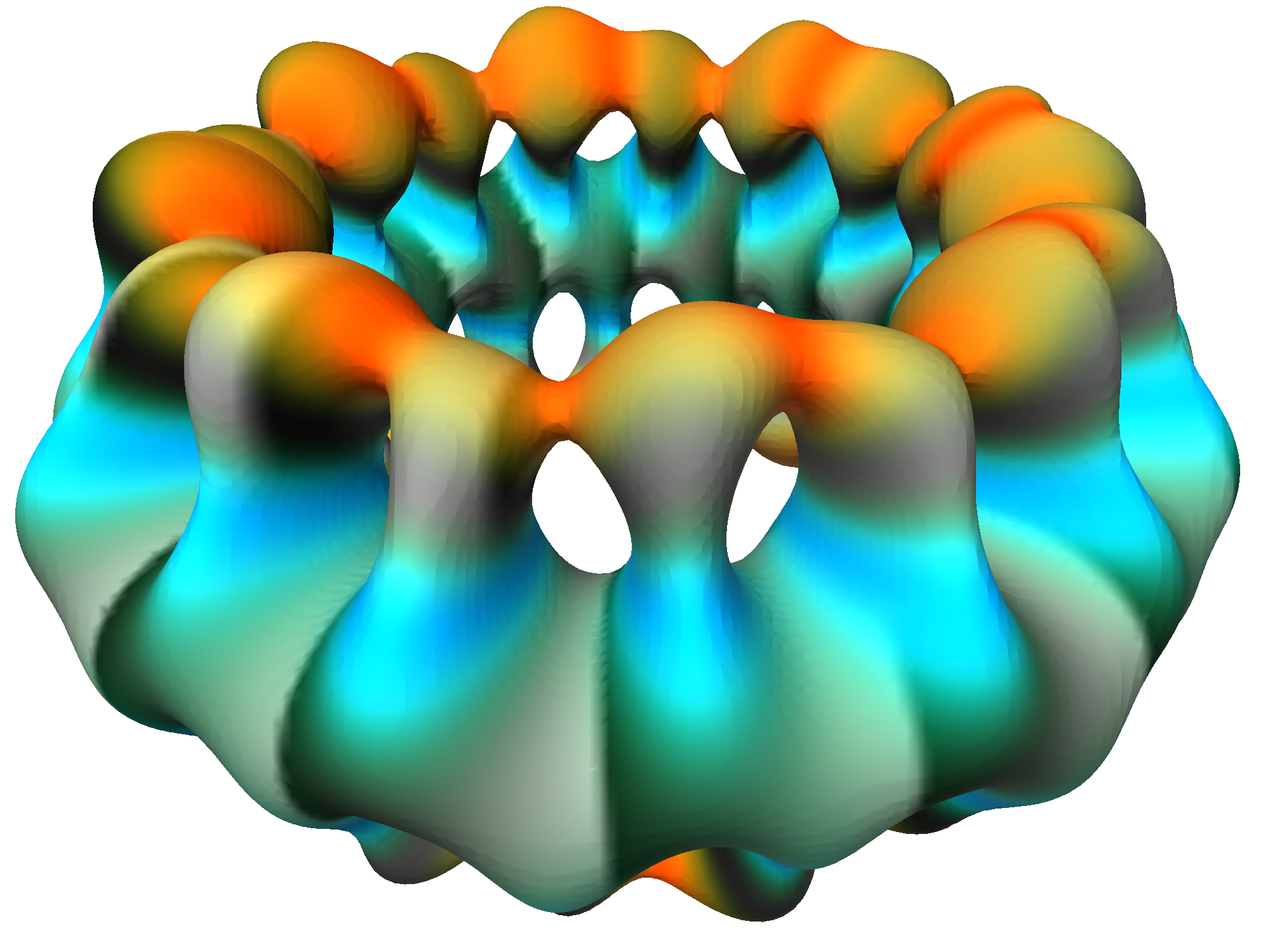
4.3 Three Eigenfunctions
Combining three eigenfunctions, each with its own frequency, yields in general a beating pattern which never reproduces itself exactly. The number of possible combinations rapidly increases, and we did not yet perform a systematic study of the resulting patterns. As with the simple combinations, the more interesting wavefunctions resulted by choosing values of n close to one another, since in this case the spatial extension of the combining eigenfunctions have a larger overlap.
A special case of physical interest is an illustration of fine-splitting of an emission spectral line. This corresponds to preparing the system in a superposition of three eigenfunctions: a low-energy eigenfunction and two ‘‘excited’’ eigenfunctions (details in Appendix). The resulting wavefunction exhibits a strong beating with a carrier frequency roughly equal to the difference between the frequencies of the excited and the low-lying eigenfunctions, slowly modulated with a frequency equal to the difference between the frequencies of the two excited eigenfunctions. Such a combination is shown in Figure
6↓. In a real physical situation the modulation is at least about 18,800 times slower than the beating frequency. Thus, if we were to rescale the involved frequencies faithfully, the modulation would be too slow to be visible. We chose therefore to rescale the frequencies independently, keeping the modulation frequency somewhat smaller than the fundamental one.
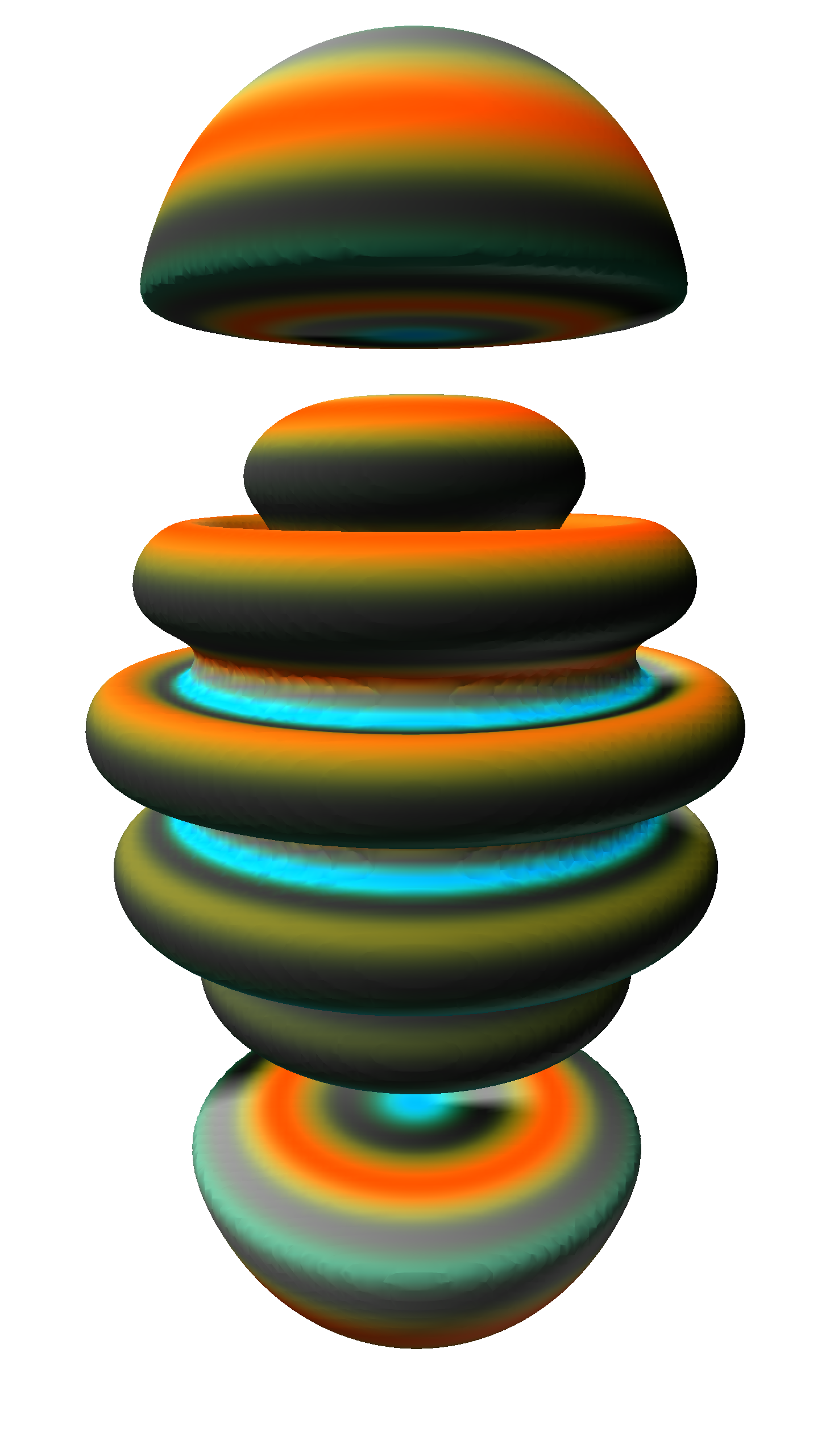
One can explore different combinations of three eigenfunctions in a similar way. Figure
7↓ shows a combination of higher-quantum number eigenfunctions, which exhibits a slow modulation of the wavefunction shape superimposed on a global rotation. These combinations would apply, e.g., to an atom immersed in a magnetic field directed along the
z-axis.
5 Future Work
5.1 Probability Flow
The evolving shape of the probability distribution is connected with the probability density flow, which demands to be visualized itself. One could achieve this by a static representation of the velocity field v(r, t), or, more intuitively, by representing via agents the actual motion with the local velocity. We have explored this option by introducing a small number of agents moving with the local velocity. The dynamics of these agents is connected to the changing shape of the wavefunction in a nontrivial and intriguing way, but a more systematic study is needed.
5.2 Time-dependent Perturbation as a Compositional Process
In order to introduce a more complex temporal behavior---like going from a fixed chord to a melody which evolves in time---one could add a time-dependent perturbation VI(t) to the Hamiltonian. This perturbation changes the wavefunction from, say, a single eigenfunction to a complex superposition of many eigenfunctions. Thus one could use in principle a well-chosen perturbation to produce a number of different wavefunctions in succession.
There are a number of technical difficulties in following this path. On the one hand, one would need enough computer power to solve the full-fledged time-dependent Schrödinger equation. One could however make the task more manageable by projecting back the evolution onto a chosen finite-dimensional subspace of wavefunctions, what allows us to exploit the already implemented representation of the wavefunctions. On the other hand, it is hard to identify which perturbation leads to a given sequence of wavefunctions. While the time-dependence of weights and phases could be chosen arbitrarily, it could be interesting to identify physically relevant perturbations which lead to interesting pattern sequences.
6 Conclusion
With the present representation of the hydrogen-like atom, we were able to study various wavefunction combinations that form “chords” from our quantum alphabet of musical “tones”. We worked together on a daily basis, eventually arriving at the current mapping representations. We implemented different iterations of the mappings, most of which were superseded as either not informative enough from the physical point of view, or not aesthetically pleasing. For example, we employed point-cloud and vector-field representations of the wavefunction, however, the visual pattern was dominated by the distribution of these reporter glyphs
[13]. The isosurface representation has the advantage of leading to an immediate grasp of the broad features of the probability density distribution described by the wavefunction. The subtler effects contained in the spinor amplitudes and phases are reasonably well reported via our color coding. We found with some satisfaction that physically-based combinations often lead to aesthetically pleasing patterns, as in the case of the light-emitting superposition.
It is easy to use the system for a visual investigation of the properties of the hydrogen atom eigenfunctions, as a function of their quantum numbers. Thus the system can be efficiently exploited as a didactic tool. However, more insight is gained by looking at the unfolding of the visual patterns of a combination of several eigenfunctions. This behavior also provides a more intuitive understanding of the mechanisms of time-dependent perturbation theory.
Appendix
A hydrogen-like atom wavefunction
Ψν(r) is given as a product of independent radial and angular functions
Ψν(r) = ⎧⎨⎩
Rn(r)Yℓm(θ, φ),
if spin is neglected,
Rn(r)ψℓJj(θ, φ, s),
with the spin
where
-
For the spinless electron: ν = (n, ℓ, m);
-
For the electron with spin: ν = (n, ℓ, J, j).
Here (r, θ, φ) are the spherical coordinates of the position r, s = ↑, ↓ is the spin quantum number, and
-
n is the principal quantum number: n = 1, 2, 3, …;
-
ℓ is the angular quantum number: ℓ = 0, 1, …, n − 1;
-
m is the magnetic quantum number: m = − ℓ, − ℓ + 1, …, ℓ − 1, ℓ;
-
J is the total angular momentum: J = ℓ±(1)/(2);
-
j is the z-component of the total angular momentum: j = − J, − J + 1, …, J − 1, J.
The wavefunctions satisfy the time-dependent Schrödinger equation
iℏ∂tΨ = ĤΨ
where the Hamiltonian operator
Ĥ corresponds to the energy of the system. The eigenfunctions
Ψν are solutions of the time-
independent Schrödinger equation
ĤΨν = ϵνΨν
and are identified by a collection
ν of quantum numbers. A general time-dependent wavefunction
Ψ is obtained as a linear combination of eigenfunctions with time-varying coefficients
cν(t) which evolve according to
cν(t) = eiϵνt ⁄ ℏcν(0).
While the amplitude
|Ψ|2 = |Ψ↑|2 + |Ψ↓|2 yields the probability of finding the electron at a given position in space, there is much physical information contained in the full
Ψ, e.g., the probability of observing a given value of the spin.
We only consider in this work pure states, which are described by a complex-valued wavefunction Ψ(x). In our case x = (r, s), so Ψ can also be considered a spinor, i.e., a two-component vector Ψ = (Ψ↑, Ψ↓). Each component of the spinor wavefunction is proportional to an eigenfunction of the spinless electron with a proportionality coefficient dictated by symmetry. Thus each spinor eigenfunction has two components, each of which is an eigenfunction of the spinless electron with different values of m. Given j, the upper and lower eigenfunctions have m = j − (1)/(2) and m = j + (1)/(2), respectively. One can associate to each spinor a 3D spin vector v which points in the local direction of the spin.
Light is emitted when the electron, coupled to an electromagnetic field, performs a transition from a state with quantum numbers ν and energy ϵν to a state with quantum numbers ν’ and a smaller energy ϵν’ (the reverse transition corresponds to light absorption). The energy of the emitted photon is given by ϵ = ϵν − ϵν’ and is related to its frequency ω by the Planck relation ϵ = ℏω. Symmetry dictates that the transition can only take place if ν and ν’ satisfy the selection rules:
-
For the spinless electron ν = (n, ℓ, m), ν’ = (n’, ℓ’, m’), with ℓ − ℓ’ = ±1, m − m’ = 0, ±1.
-
For the electron with spin, ν = (n, ℓ, J, j), ν’ = (n’, ℓ’, J’, j’), with ℓ − ℓ’ = ±1, j − j’ = 0, ±1.
Fine-splitting of an emission spectral line corresponds to a superposition of three eigenfunctions: a low-lying eigenfunction with quantum numbers (n0, ℓ0, J0), and two ‘‘excited’’ eigenfunctions with n1, 2 = n0, ℓ1, 2 = ℓ0 + 1 and two different values J1 and J2 satisfying J1, 2 = ℓ±(1)/(2).
Acknowledgments
This material is based upon work supported by the National Science Foundation under Grant Numbers 0821858, 0855279, and IIS-1047678.
References
[1] AlloSphere Research Group, “AlloSystem”. 2013. URL http://github.com/AlloSphere-Research-Group/AlloSystem.
[2] Xavier Amatriain, JoAnn Kuchera-Morin, Tobias Hollerer, Stephen Travis Pope, “The AlloSphere: Immersive Multimedia for Scientific Discovery and Artistic Exploration”, IEEE MultiMedia, vol. 16, no. 2, pp. 64—75, 2009.
[3] Bernd Thaller, Advanced Visual Quantum Mechanics. Springer Science, 2005.
[4] Bernd Thaller, Visual Quantum Mechanics. Springer TELOS, 2000.
[5] David Joiner, “Visualization of Hydrogen Lesson”. 2008. URL http://www.shodor.org/refdesk/Resources/Activities/VisHydrogen/lesson.php.
[6] Dean E. Dauger, “Real-time Visualizations of Quantum Atomic Orbitals”. 2001. URL http://daugerresearch.com/orbitals/index.shtml.
[7] H. E. White, “Pictorial Representations of the Electron Cloud for Hydrogen-like Atoms”, Physical Review, vol. 37, no. 11, pp. 1416-1424, 1931.
[8] H. Schenker, Free Composition (Der Freie Satz): Volume III of New Musical Theories and Fantasies. Schirmer, 1979.
[9] Hans Lundmark, “Visualizing Complex Analytic Functions Using Domain Coloring”. 2004. URL http://www.mai.liu.se/~alun/complex/domain_coloring-unicode.html.
[10] Iannis Xenakis, Formalized Music: Thought and Mathematics in Music. Pendragon Press, 1992.
[11] John Whitney, Digital Harmony: On the Complementarity of Music and Visual Art. Kingsport Press, 1980.
[12] Julian Voss-Andreae, “Quantum Sculpture: Art Inspired by the Deeper Nature of Reality”, Leonardo, vol. 44, no. 1, pp. 14-20, 2011.
[13] J. Kuchera-Morin, L. J. Putnam, G. Wakefield, H. Ji, B. Alper, D. Adderton, “Immersed in Unfolding Complex Systems”. 2010.
[14] JoAnn Kuchera-Morin, “Performing in Quantum Space: A Creative Approach to N-Dimensional Computing”, Leonardo Journal, vol. 44, no. 5, pp. 462—463, 2011.
[15] M. Belloni, W. Christian, “Time development in quantum mechanics using a reduced Hilbert space approach”, American Journal of Physics, vol. 76, no. 4, pp. 385, 2008.
[16] Mario Belloni, Wolfgang Christian, “OSP-based Programs for Quantum Mechanics: Time Evolution and ISW Revivals”. 2004. URL http://www.phy.davidson.edu/FacHome/mjb/xml_qm/default.html.
[17] Paul Falstad, “Hydrogen Atom Orbital Viewer”. 2005. URL http://www.falstad.com/qmatom/.
[18] Siegmund Brandt, Hans Dieter Dahmen, T. Stroh, Interactive Quantum Mechanics: Quantum Experiments on the Computer. Springer, 2011.
Glossary
Eigenfunction In quantum mechanics, a wavefunction associated with a specific possible value of a physical observable. A general wavefunction can be obtained as a superposition of eigenfunctions.
Perceptualization The mapping of data so that it can be perceived in a meaningful way through human senses, e.g., visualization and sonification.
Pure state A state of a quantum system which contains its fullest specification compatible with the laws of quantum mechanics. It is described by a wavefunction.
Schrödinger equation The equation describing the evolution of a quantum state. It reads iℏ∂tΨ = Ĥ Ψ, where Ĥ is the Hamiltonian operator associated with the energy of the system.
Spin A purely quantum degree of freedom of elementary particles, representing an intrinsic contribution to the total angular momentum. For electrons, the spin assumes the values ±ℏ ⁄ 2, where ℏ is the reduced Planck constant.
Superposition An additive mixture of waveforms, typically from the same family of functions. The parts cannot necessarily be recovered fully from the whole. The solutions of the Schrödinger equation are a superposition of eigenfunctions with time-varying coefficients.
Wavefunction The complex-valued function Ψ(x), defined on the configuration space of a quantum system, which contains a full description of a pure quantum state. Its evolution is described by the time-dependent Schrödinger equation.